Most simple graphs generally include graphical representation of data using various plot type such as bar charts, scatter plots, histograms, box plots step plots and more. Both SG procedures and GTL provide many easy ways to create such graphs.
However, for many real world use cases, we need to display related textual data in the graph, usually aligned with one of the axes. Over the past few years with SAS 9.2 we have done this using the SCATTER plot with the MARKERCHARACTER option. This option displays the textual value from the associated column in the (x, y) location in place of a marker. This text string is center-justified at the marker location. While this works for many cases, sometimes we need finer control over the placement of the text.
Recently a SAS user posted just such a question on the SAS Communities page. User wanted the text to be left justified, using SAS 9.3 and was looking for some help. With SAS 9.2, one has to use the MARKERCHARACTER option and then use some coding tricks to position the strings just right. I have discuss some ways earlier using Non-Breaking Spaces.
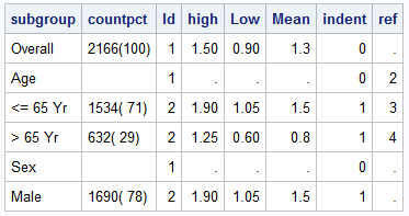
With SAS 9.3, there are some more options available to user, and I thought this would make for a good blog article. Let us use the data in the article Forest Plot with SAS 9.3 to illustrate the possibilities. We will use only the columns on the left and the hazard plot. Note in this data set, the observations with ID=1 are subgroup headings and the observations with ID=2 are the values. The intention is to display the subgroup headings with bolder fonts and the values with an indentation.
We can use a two cell lattice and populate the first cell with the first two columns from this data set. The second cell will contain a scatter plot of the mean with low and high limits by study. Here is the graph using the MarkerCharacter option. Click on the graph for a high resolution graph.

Here is the code fragment for the first cell in the graph. Please see the full code in the attached program file.
  layout overlay / walldisplay=none
               x2axisopts=(display=(tickvalues) offsetmin=0.3 offsetmax=0.3
               yaxisopts=(reverse=true display=none offsetmin=0);
    scatterplot y=obsid x=subgroup_lbl / markercharacter=subgroup xaxis=x2;
    scatterplot y=obsid x=count_lbl / markercharacter=countpct xaxis=x2;
endlayout; |
In the graph above, the textual data is positioned center-justified for each text string. This is not what we want. To address this, some suggestions were made in the blog posts referred above. The solutions are not optimal, and require the use of non-proportional fonts.
The SCATTER plot also supports another way to display text data using the DATALABEL option. With SAS 9.2, this data label is always displayed at the top right of the marker, and can be moved around by the system to avoid collisions with other labels or markers. So, with SAS 9.2, it was not possible to use this feature to draw the text strings with deterministic results. However, with SAS 9.3, a new DATALABELPOSITION option is added, allowing explicit positioning of the labels. While the default position is AUTO, meaning the old collision avoidance behavior, you can also specify any compass position such as TOP, LEFT, etc.
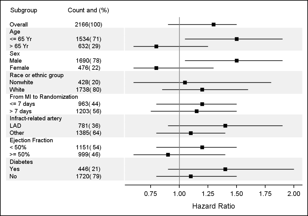
In the graph below, we have used the DATALABEL option to display the text, using DATALABELPOSITION of RIGHT and CENTER. RIGHT places the text to the right of the invisible marker, effectively making the text left justified.
Here is the SAS 9.3 code fragment for the first cell.
  layout overlay / walldisplay=none
                   x2axisopts=(display=(tickvalues) offsetmin=0.15 offsetmax=0.3
                   yaxisopts=(reverse=true display=none offsetmin=0);
    scatterplot y=obsid x=subgroup_lbl / datalabel=subgroup markerattrs=(size=0)
                datalabelposition=right xaxis=x2 discreteoffset=-0.25;
    scatterplot y=obsid x=count_lbl / datalabel=countpct markerattrs=(size=0)
                datalabelposition=center xaxis=x2;
endlayout; |
This is an improvement over the first graph, but the observations like "Overall", "Age", "Sex" are subgroups, and we want to display them in bold, and the observations like "<= 65 yr" etc. are values which we want to display indented over a bit. How can we do that?
One way with SAS 9.3 GTL is to use the EVAL function to have a scatter plot display only the values with ID=1 with specified attributes, and another scatter plot display only the values with ID=2 using different attributes and offset. Here is the result:
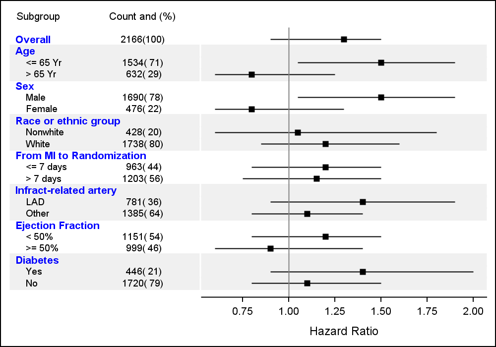
Note, in this case all the subgroup headings (ID=1) are displayed with a blue bold font of size 8 while the values are displayed with normal font with an offset using the DISCRETEOFFSET option. Here is the SAS 9.3 GTL code fragment.
  layout overlay / walldisplay=none
               x2axisopts=(display=(tickvalues) offsetmin=0.15 offsetmax=0.3
               yaxisopts=(reverse=true display=none offsetmin=0);
    scatterplot y=eval(ifn(id=1, obsid, .)) x=subgroup_lbl / datalabel=subgroup
                markerattrs=(size=0) datalabelposition=right xaxis=x2
                discreteoffset=-0.25 datalabelattrs=(weight=bold size=8  color=blue);
    scatterplot y=eval(ifn(id=2, obsid, .)) x=subgroup_lbl / datalabel=subgroup
                markerattrs=(size=0) datalabelposition=right
                xaxis=x2 discreteoffset=-0.15 datalabelattrs=(weight=normal size=7);
    scatterplot y=obsid x=count_lbl / datalabel=countpct markerattrs=(size=0)
                datalabelposition=center xaxis=x2 datalabelattrs=(size=7);
endlayout; |
Note, now we are using two scatter plots to display the first column. The first one displays only the observations with ID=1 (the subgroup headings) with a blue bold font. The second one displays only the observations with ID=2 (the values) with a normal font with an offset. Note the use of the Y=EVAL(IFN ( ) ) expressions.
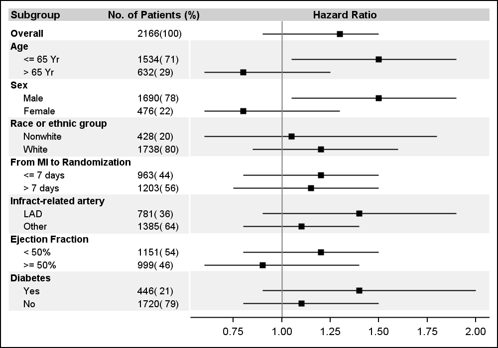
With SAS 9.2 and SAS 9.3 we found ourselves doing this so often, that we decided we needed a special statement to make it easy to display such columns (or rows) of textual data axis aligned with the Y or X axis. So, with SAS 9.4 is included a new plot statement AXISTABLE. This statement makes it very easy to create such textual entries, and supports text attributes and indentation. Here is the resulting graph using SAS 9.4 AXISTABLE:
Here is the SAS 9.4 code fragment to create the text data columns:
layout overlay / yaxisopts=(reverse=true display=none offsetmin=0) walldisplay=none; innermargin / align=left opaque=false; axistable y=obsid value=subgroup / indentweight=indent textgroup=textid; axistable y=obsid value=countpct / labelattrs=(size=7); endinnermargin; endlayout; |
Note the use of INDENTWEIGHT and TEXTGROUP for the first column. These axis table statements are placed in the INNERMARGIN, which automatically computes the amount of space needed for each column. With SAS 9.4, you can now have inner margins on left and right of the overlay container.
Full SAS code (SAS 9.3 and SAS 9.4): DataLabels


4 Comments
Thanks for the help with this and the further improvement looks great...I'll put the bolding in too.
Pingback: Graph Table - Graphically Speaking
Hi
Thank you for the tip but I need some help from you.
When I run the following code:
data DATA;
input GENDER $ 1-6 REFERANSE_PCT 8-11 MALGRUPPE_PCT 13-16 N_REF 18-23 N_MAL 25-30 AVVIK 32-36 GROUP $38-45 CONSTANT 47 REFERANSE_N_LBL $49-53 MALGRUPPE_N_LBL $55-60 OBSID 61;
datalines;
0 0 100 0 0 Negative 0 N_REF N_MAL 1
Kvinne 0.52 0.40 50000 100000 -0.24 Negative 0 N_REF N_MAL 2
Mann 0.48 0.60 135967 31527 0.26 Positive 0 N_REF N_MAL 3
;
run;
ods graphics on / width=1145px height=630px; * Fit to PowerPoint slide ;
proc template;
define statgraph PROFILE;
* dynamic _bandcolor;
begingraph / includemissingdiscrete=true;
dynamic var;
entrytitle "GENDER";
layout lattice / columns=2 columngutter=2 columnweights=(0.3 0.7);
/*--First column for Subgroup and patient counts--*/
layout overlay / walldisplay=none border=false
x2axisopts=(display=(tickvalues) offsetmin=0 offsetmax=0.6 tickvalueattrs=(size=12pt weight=bold))
yaxisopts=(reverse=true display=none tickvalueattrs=(weight=bold) offsetmin=0);
* referenceline y=ref / lineattrs=(thickness=14 color=_bandcolor);
scatterplot y=obsid x=referanse_n_lbl / datalabel=N_REF markerattrs=(size=0) datalabelposition=right datalabelattrs=( size=12pt weight=bold)
xaxis=x2 discreteoffset=-.35;
scatterplot y=obsid x=malgruppe_n_lbl / datalabel=N_MAL markerattrs=(size=0) datalabelposition=right datalabelattrs=( size=12pt weight=bold) xaxis=x2;
endlayout;
layout overlay / xaxisopts=( TICKVALUEATTRS=(SIZE=12pt) griddisplay=on Label="% av målgruppe" /*offsetmin=0*/ type=linear ) yaxisopts= (TICKVALUEATTRS=(SIZE=12pt) reverse=true display=( ticks tickvalues line ) type=discrete ) y2axisopts=(reverse=true);
if (_NEGATIVE_) ReferenceLine x=0 / lineattrs=GraphAxisLines;
endif;
barchart X=GENDER Y=MALGRUPPE_PCT / primary=true orient=horizontal LegendLabel=" " NAME="a" /*dataskin=PRESSED*/ target=REFERANSE_PCT barlabel=true barlabelattrs=(size=12pt) barwidth=0.6 ;
/*ScatterPlot X='TARGET'n Y='CU_GENDER'n / discreteOffset=-0.35 Markerattrs=( Symbol=TRIANGLEDOWNFILLED Size=10) DataTransparency=0.4 LegendLabel="normale population" NAME="t";*/
/* DiscreteLegend "a" "t" / Location=outside Title="";*/
endlayout;
endlayout;
endgraph;
end;
run;
*ods graphics / reset width=5in height=3.5in imagename='PROFILE';
proc sgrender data=WORK.DATA template=PROFILE;
*dynamic _bandcolor='cxf0f0f0';
dynamic var="GENDER" ;
format MALGRUPPE_PCT percent12.1 N_MAL N_REF COMMAX15.;
run;
You will see that N_REF and N_MAL are out of place and the numbers are centered even though I have used datalabelposition=right. There are many things I do not understand here.
Any help is appriciated.
Thanks
best regards
Johan
Hi
Thank you for the tip but I need some help from you.
When I run the following code:
data DATA;
input GENDER $ 1-6 REFERANSE_PCT 8-11 MALGRUPPE_PCT 13-16 N_REF 18-23 N_MAL 25-30 AVVIK 32-36 GROUP $38-45 CONSTANT 47 REFERANSE_N_LBL $49-53 MALGRUPPE_N_LBL $55-60 OBSID 61;
datalines;
0 0 100 0 0 Negative 0 N_REF N_MAL 1
Kvinne 0.52 0.40 50000 100000 -0.24 Negative 0 N_REF N_MAL 2
Mann 0.48 0.60 135967 31527 0.26 Positive 0 N_REF N_MAL 3
;
run;
ods graphics on / width=1145px height=630px; * Fit to PowerPoint slide ;
proc template;
define statgraph PROFILE;
* dynamic _bandcolor;
begingraph / includemissingdiscrete=true;
dynamic var;
entrytitle "GENDER";
layout lattice / columns=2 columngutter=2 columnweights=(0.3 0.7);
/*--First column for Subgroup and patient counts--*/
layout overlay / walldisplay=none border=false
x2axisopts=(display=(tickvalues) offsetmin=0 offsetmax=0.6 tickvalueattrs=(size=12pt weight=bold))
yaxisopts=(reverse=true display=none tickvalueattrs=(weight=bold) offsetmin=0);
* referenceline y=ref / lineattrs=(thickness=14 color=_bandcolor);
scatterplot y=obsid x=referanse_n_lbl / datalabel=N_REF markerattrs=(size=0) datalabelposition=right datalabelattrs=( size=12pt weight=bold)
xaxis=x2 discreteoffset=-.35;
scatterplot y=obsid x=malgruppe_n_lbl / datalabel=N_MAL markerattrs=(size=0) datalabelposition=right datalabelattrs=( size=12pt weight=bold) xaxis=x2;
endlayout;
layout overlay / xaxisopts=( TICKVALUEATTRS=(SIZE=12pt) griddisplay=on Label="% av målgruppe" /*offsetmin=0*/ type=linear ) yaxisopts= (TICKVALUEATTRS=(SIZE=12pt) reverse=true display=( ticks tickvalues line ) type=discrete ) y2axisopts=(reverse=true);
if (_NEGATIVE_) ReferenceLine x=0 / lineattrs=GraphAxisLines;
endif;
barchart X=GENDER Y=MALGRUPPE_PCT / primary=true orient=horizontal LegendLabel=" " NAME="a" /*dataskin=PRESSED*/ target=REFERANSE_PCT barlabel=true barlabelattrs=(size=12pt) barwidth=0.6 ;
/*ScatterPlot X='TARGET'n Y='CU_GENDER'n / discreteOffset=-0.35 Markerattrs=( Symbol=TRIANGLEDOWNFILLED Size=10) DataTransparency=0.4 LegendLabel="normale population" NAME="t";*/
/* DiscreteLegend "a" "t" / Location=outside Title="";*/
endlayout;
endlayout;
endgraph;
end;
run;
*ods graphics / reset width=5in height=3.5in imagename='PROFILE';
proc sgrender data=WORK.DATA template=PROFILE;
*dynamic _bandcolor='cxf0f0f0';
dynamic var="GENDER" ;
format MALGRUPPE_PCT percent12.1 N_MAL N_REF COMMAX15.;
run;
You will see that N_REF and N_MAL are out of place and the numbers are centered even though I have used datalabelposition=right. There are many things I do not understand here.
Any help is appreciated.
Thanks
best regards
Johan